
【Rでベイズ統計モデリング#15】ランダム係数モデル(brms)
記事の目的
GLMであるランダム係数モデルのベイズ推定を、RとStanを使用して実装していきます。今回は、「brms」というライブラリを使用します。データの作成から実装するので、コピペで再現することが可能です。
目次
0 前準備
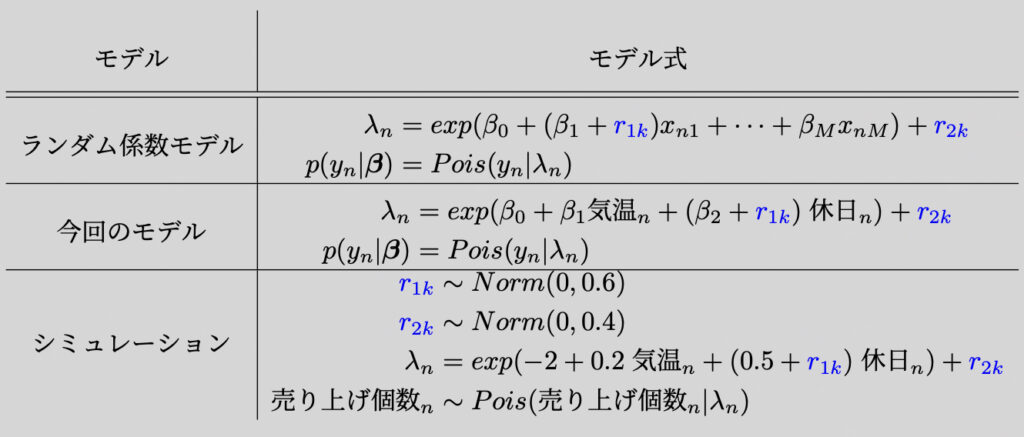
0.1 今回のモデル
0.2 ワーキングディレクトリの設定
以下の画像のようにワーキングディレクトリを設定します。設定したディレクトリに、RファイルとStanファイルを保存します。

1 ライブラリ
# 1 ライブラリ
library(dplyr)
library(ggplot2)
library(rstan)
library(brms)
library(patchwork)

set.seed(1)
rstan_options(auto_write=TRUE)
options(mc.cores=parallel::detectCores())
2 データ
2.1 コード
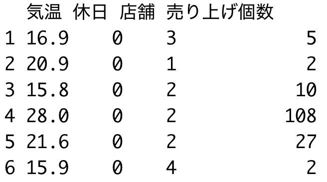
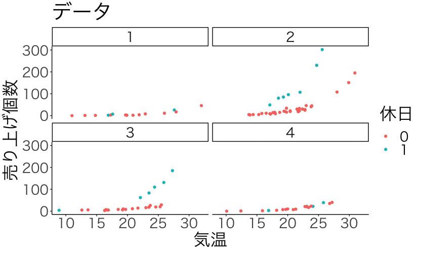
# 2 データ
気温 <- rnorm(100,20,5) %>% round(1)
休日 <- rbinom(100, 1, 2/7)
店舗 <- runif(100, 1, 4) %>% round()
r1 <- rnorm(4, 0, 0.6)
r2 <- rnorm(4, 0, 0.4)
data <- data.frame(気温, 休日, 店舗) %>%
  mutate(r1=ifelse(店舗==1, r1[1], ifelse(店舗==2, r1[2], ifelse(店舗==3, r1[3],r1[4]))))%>%
  mutate(r2=ifelse(店舗==1, r2[1], ifelse(店舗==2, r2[2], ifelse(店舗==3, r2[3],r2[4]))))%>%
  mutate(lambda=exp(-2+0.2*気温+(0.5+r1)*休日+r2)) %>%
  mutate(休日=factor(休日))
data$売り上げ個数 <- rpois(100, data$lambda)
data %>% select(気温, 休日, 店舗, 売り上げ個数) %>% head()

plot <- data %>%
  ggplot(aes(x=気温, y=売り上げ個数, color=休日)) +
  geom_point() +
  theme_classic(base_family = "HiraKakuPro-W3") +
  theme(text=element_text(size=25))+
  labs(x="気温", y="売り上げ個数", title="データ") +
  facet_wrap(.~ 店舗)
plot
2.2 結果
| 13行目の結果 | 22行目の結果 |
 |
 |
3 brmsの利用
# 3 brmsの使用
mcmc_result <- brm(
  data = data,
  formula = 売り上げ個数~ 気温 + 休日 + (休日||店舗),
  family = poisson(),
  seed = 1,
  iter = 2000, warmup = 200, chains = 4, thin=1
)
4 分析結果
4.1 コード
# 4 分析結果
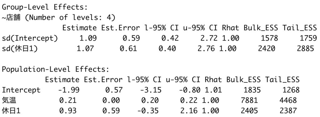
## 4.1 推定結果
print(mcmc_result)
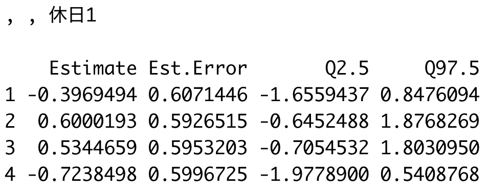
ranef(mcmc_result)
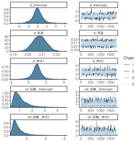
## 4.2 収束の確認
theme_set(theme_classic(base_size = 10, base_family = "HiraKakuProN-W3"))
plot(mcmc_result)
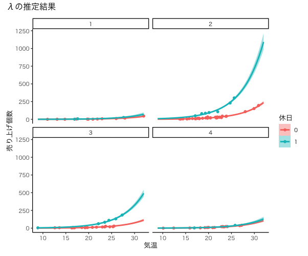
## 4.3 λの確認
condition <- data.frame(店舗=1:4)
plot(conditional_effects(mcmc_result, effects="気温:休日",re_formula=NULL,
conditions = condition), points=TRUE, ncol=2) %>%
wrap_plots() + plot_annotation(title="λの推定結果")
## 4.4 予測分布
plot(conditional_effects(mcmc_result, effects="気温:休日",re_formula=NULL,
conditions = condition, method="predict"), points=TRUE, ncol=2)%>%
wrap_plots() + plot_annotation(title="予測分布")
4.2 結果
| 3行目の結果 | 8行目の結果 |
|
 |
| 12行目の結果 | 17行目の結果 |
 |
 |