【Rでベイズ統計モデリング#19】ローカル線形トレンドモデル

記事の目的

状態空間モデルであるローカル線形トレンドモデルのベイズ推定を、RとStanを使用して実装していきます。データの作成から実装するので、コピペで再現することが可能です。

0 前準備

0.1 今回のモデル

0.2 ワーキングディレクトリの設定

以下の画像のようにワーキングディレクトリを設定します。設定したディレクトリに、RファイルとStanファイルを保存します。

1 ライブラリ

# 1 ライブラリ
library(dplyr)
library(ggplot2)
library(rstan)
library(bayesplot)
library(gridExtra)

set.seed(2)
rstan_options(auto_write=TRUE)
options(mc.cores=parallel::detectCores())

2 データ

2.1 コード

# 2 データ
## 2.1 データの作成
日付 <- seq(as.POSIXct("2021/05/01"), as.POSIXct("2021/08/01"), "days")
売り上げ <- c()
mu <- c()
delta <- c()
mu[1] <- rnorm(1, 20, 1) %>% round(1)
delta[1] <- rnorm(1, 5, 1) %>% round(1)
T <- length(日付)
for(t in 2:T){
  delta[t] <- rnorm(1, delta[t-1], 2)
  mu[t] <- rnorm(1, mu[t-1]+delta[t-1], 5)
}
for(t in 1:T){
  売り上げ[t] <- rnorm(1, mu[t], 3) 
}
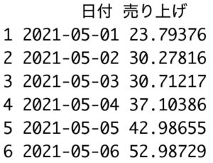
data <- data.frame(日付, 売り上げ)
data %>% head()

## 2.2 データの可視化
plot <- data %>% 
  ggplot(aes(x=日付)) +
  theme_classic(base_family = "HiraKakuPro-W3") +
  theme(text = element_text(size = 20))+
  scale_x_datetime(date_labels = "%m/%d")

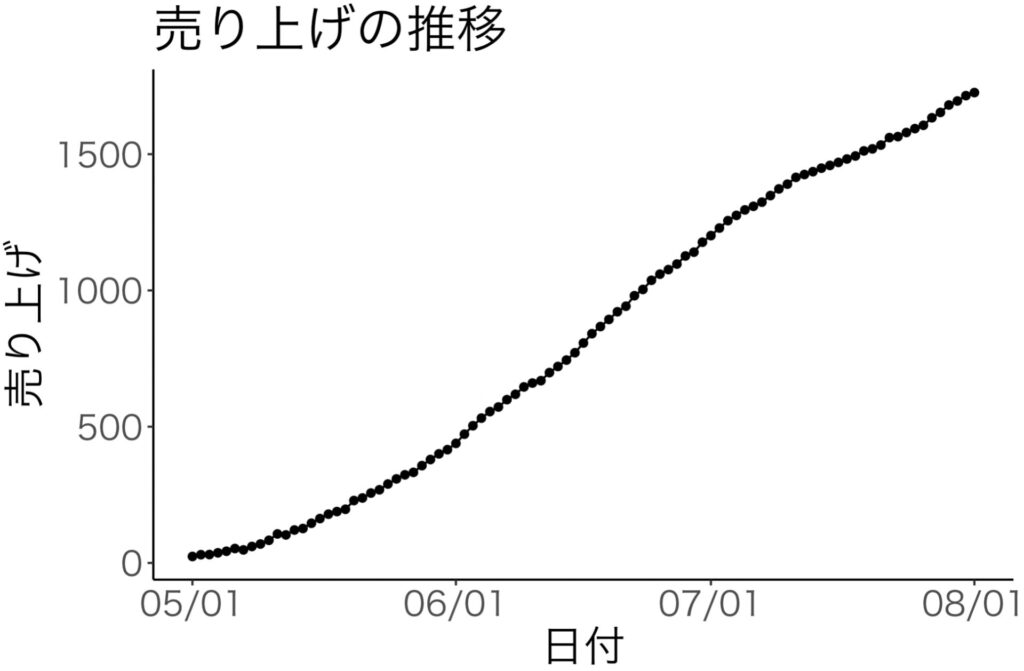
plot + 
  geom_point(aes(y=売り上げ))+
  geom_line(aes(y=売り上げ)) +
  labs(x="日付",y="売り上げ",title="売り上げの推移")

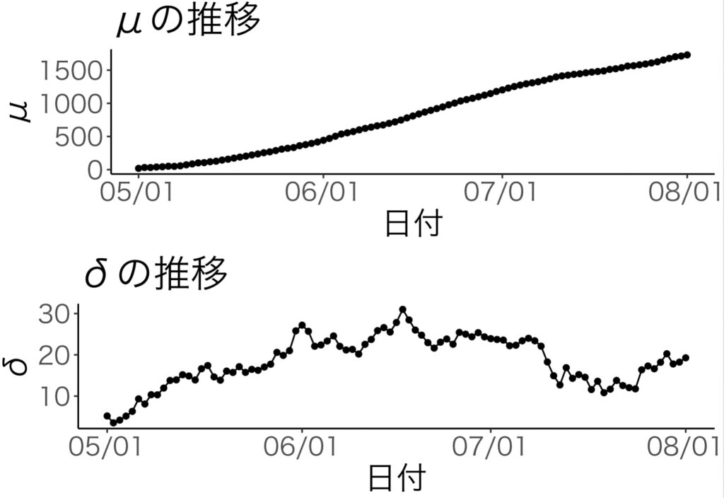
## 2.3 パラメータの可視化
plot_mu_sim <- plot + 
  geom_point(aes(y=mu))+
  geom_line(aes(y=mu)) +
  labs(x="日付",y="μ",title="μの推移")

plot_delta_sim <- plot + 
  geom_point(aes(y=delta))+
  geom_line(aes(y=delta)) +
  labs(x="日付",y="δ",title="δの推移")

grid.arrange(plot_mu_sim, plot_delta_sim)

2.2 結果

18行目の結果

27行目の結果	43行目の結果

3 Stanの利用

3.1 Stanファイル

data {
  int T;
  vector[T] y;
}

parameters {
  vector[T] mu;
  vector[T] delta;
  real<lower=0> sigma_w;
  real<lower=0> sigma_v;
  real<lower=0> sigma_d;
}

model {
  delta[2:T] ~ normal(delta[1:(T-1)], sigma_d);
  mu[2:T] ~ normal(mu[1:(T-1)]+delta[1:(T-1)], sigma_w);
  y ~ normal(mu, sigma_v);
}

generated quantities{
  vector[T] y_pred;
  for(t in 1:T){
    y_pred[t] = normal_rng(mu[t], sigma_v);
  }
}

3.2 Stanを利用するRのコード

# 3 stanの利用
data_list <- list(
  T = nrow(data),
  y = data$売り上げ
)

mcmc_result <- stan(
  file="19ローカル線形トレンドモデル.stan",
  data=data_list,
  seed=1,
  iter = 2000, warmup = 200, chains = 3, thin=1
)

4 分析結果

4.1 コード

# 4 分析結果
## 4.1 推定結果
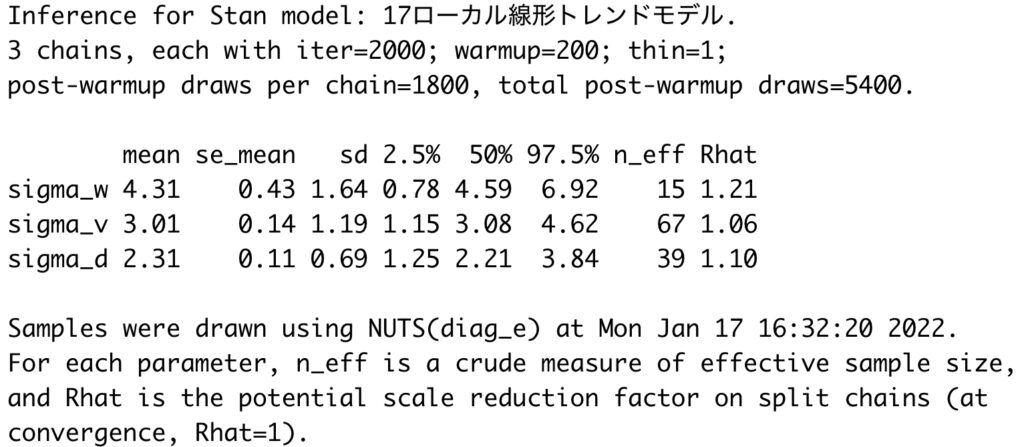
print(mcmc_result, pars=c("sigma_w", "sigma_v", "sigma_d"), probs = c(0.025, 0.5, 0.975))

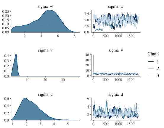
## 4.2 収束の確認
mcmc_sample <- rstan::extract(mcmc_result, permuted=FALSE)
mcmc_combo(mcmc_sample, pars=c("sigma_w","sigma_v","sigma_d"))

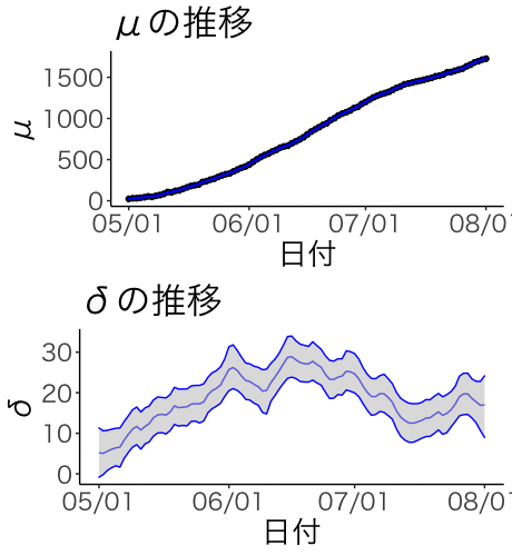
## 4.3パラメータの確認
mcmc_sample <- rstan::extract(mcmc_result)
func <- function(x){
  return (quantile(x, c(0.025, 0.5, 0.975)))
}
mu <- apply(mcmc_sample[["mu"]], 2, func)
plot_mu <- plot + 
  geom_point(aes(y=売り上げ))+
  geom_line(aes(y=mu[2,]), col="blue") + 
  geom_ribbon(aes(ymin=mu[1,],ymax=mu[3,]), alpha=0.5, fill="gray", col="blue") +
  labs(x="日付",y="μ",title="μの推移")

delta <- apply(mcmc_sample[["delta"]], 2, func)

plot_delta <- plot + 
  geom_line(aes(y=delta[2,]), col="blue") + 
  geom_ribbon(aes(ymin=delta[1,],ymax=delta[3,]), alpha=0.5, fill="gray", col="blue") +
  labs(x="日付",y="δ",title="δの推移")

grid.arrange(plot_mu, plot_delta)

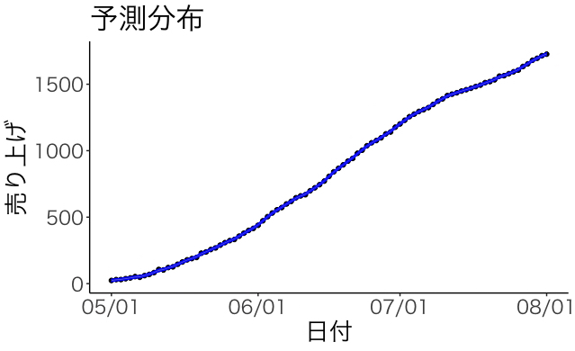
## 4.4 予測分布
y_pred <- apply(mcmc_sample[["y_pred"]], 2, func)

plot + 
  geom_point(aes(y=売り上げ))+
  geom_line(aes(y=y_pred[2,]), col="blue") + 
  geom_ribbon(aes(ymin=y_pred[1,],ymax=y_pred[3,]), alpha=0.5, fill="gray", col="blue") +
  labs(x="日付",y="売り上げ",title="予測分布")