
【pytorchで深層生成モデル#5】pytorchでVAE
記事の目的
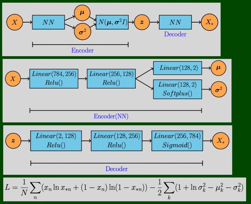
深層生成モデルのVAE(Variable Auto Encoder)をpytorchを使用して実装していきます。ここにある全てのコードは、コピペで再現することが可能です。
目次
1 今回のモデル
2 準備

# [1]
!nvidia-smi
# [2]
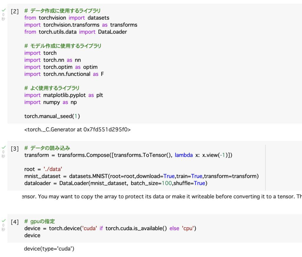
# データ作成に使用するライブラリ
from torchvision import datasets
import torchvision.transforms as transforms
from torch.utils.data import DataLoader
# モデル作成に使用するライブラリ
import torch
import torch.nn as nn
import torch.optim as optim
import torch.nn.functional as F
# よく使用するライブラリ
import matplotlib.pyplot as plt
import numpy as np
torch.manual_seed(1)
# [3]
# データの読み込み
transform = transforms.Compose([transforms.ToTensor(), lambda x: x.view(-1)])
root = './data'
mnist_dataset = datasets.MNIST(root=root,download=True,train=True,transform=transform)
dataloader = DataLoader(mnist_dataset, batch_size=100,shuffle=True)
# [4]
# gpuの指定
device = torch.device('cuda' if torch.cuda.is_available() else 'cpu')
device
3 モデル
# [5]
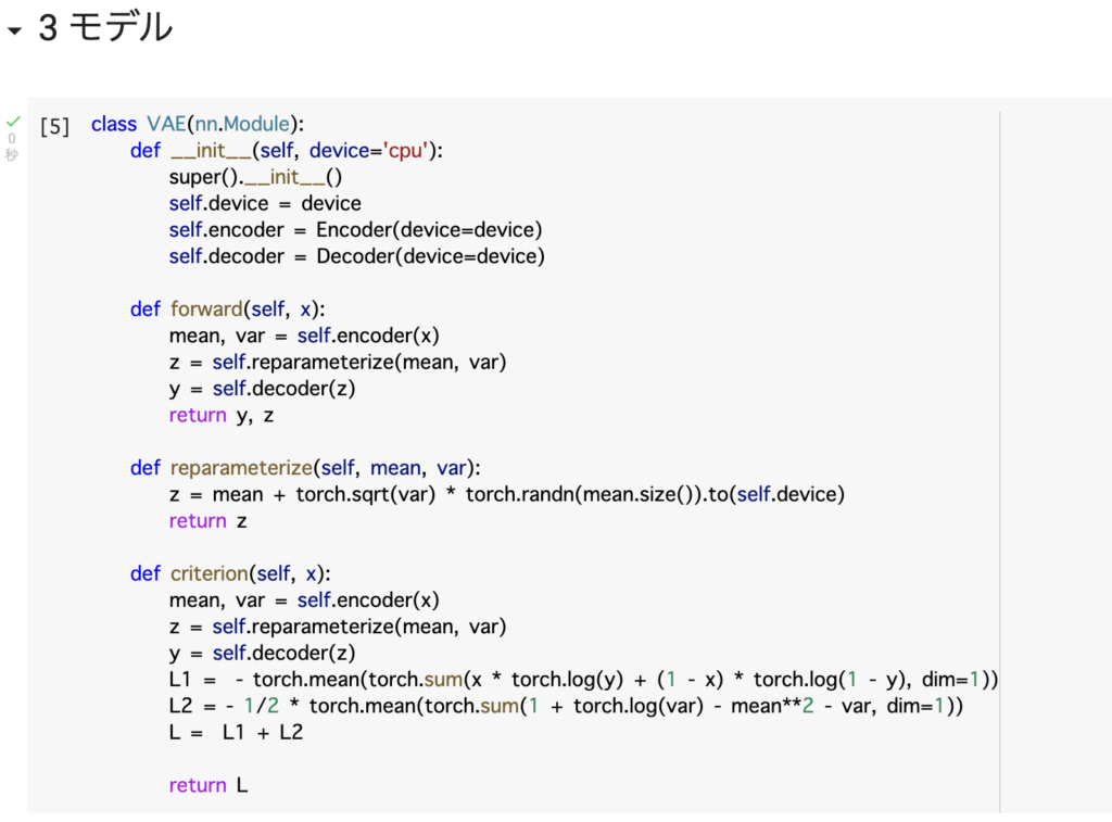
class VAE(nn.Module):
def __init__(self, device='cpu'):
super().__init__()
self.device = device
self.encoder = Encoder(device=device)
self.decoder = Decoder(device=device)
def forward(self, x):
mean, var = self.encoder(x)
z = self.reparameterize(mean, var)
y = self.decoder(z)
return y, z
def reparameterize(self, mean, var):
z = mean + torch.sqrt(var) * torch.randn(mean.size()).to(self.device)
return z
def criterion(self, x):
mean, var = self.encoder(x)
z = self.reparameterize(mean, var)
y = self.decoder(z)
L1 = - torch.mean(torch.sum(x * torch.log(y) + (1 - x) * torch.log(1 - y), dim=1))
L2 = - 1/2 * torch.mean(torch.sum(1 + torch.log(var) - mean**2 - var, dim=1))
L = L1 + L2
return L
# [6]
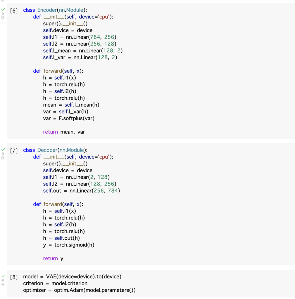
class Encoder(nn.Module):
def __init__(self, device='cpu'):
super().__init__()
self.device = device
self.l1 = nn.Linear(784, 256)
self.l2 = nn.Linear(256, 128)
self.l_mean = nn.Linear(128, 2)
self.l_var = nn.Linear(128, 2)
def forward(self, x):
h = self.l1(x)
h = torch.relu(h)
h = self.l2(h)
h = torch.relu(h)
mean = self.l_mean(h)
var = self.l_var(h)
var = F.softplus(var)
return mean, var
# [7]
class Decoder(nn.Module):
def __init__(self, device='cpu'):
super().__init__()
self.device = device
self.l1 = nn.Linear(2, 128)
self.l2 = nn.Linear(128, 256)
self.out = nn.Linear(256, 784)
def forward(self, x):
h = self.l1(x)
h = torch.relu(h)
h = self.l2(h)
h = torch.relu(h)
h = self.out(h)
y = torch.sigmoid(h)
return y
# [8]
model = VAE(device=device).to(device)
criterion = model.criterion
optimizer = optim.Adam(model.parameters())
4 モデルの学習
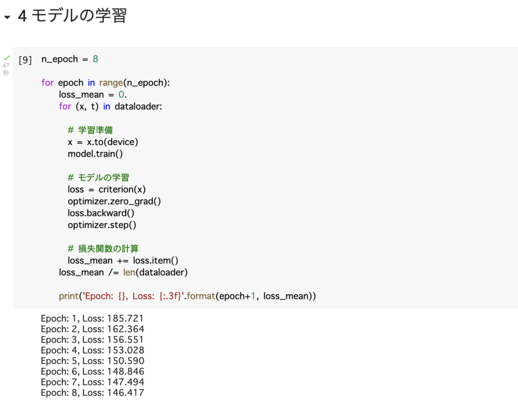
# [9]
n_epoch = 8

for epoch in range(n_epoch):
    loss_mean = 0.
    for (x, t) in dataloader:

      # 学習準備
      x = x.to(device)
      model.train()

      # モデルの学習
      loss = criterion(x)
      optimizer.zero_grad()
      loss.backward()
      optimizer.step()

      # 損失関数の計算
      loss_mean += loss.item()
    loss_mean /= len(dataloader)

    print('Epoch: {}, Loss: {:.3f}'.format(epoch+1, loss_mean))
5 画像の生成


# [10]
# データの生成
model.eval()
z = torch.randn(10, 2, device = device)
images = model.decoder(z)
images = images.view(-1, 28, 28)
images = images.squeeze().detach().cpu().numpy()
# データの可視化
for i, image in enumerate(images):
plt.subplot(2, 5, i+1)
plt.imshow(image, cmap='binary_r')
plt.axis('off')
plt.tight_layout()
plt.show()
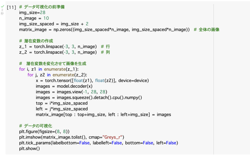
# [11]
# データ可視化の前準備
img_size=28
n_image = 10
img_size_spaced = img_size + 2
matrix_image = np.zeros((img_size_spaced*n_image, img_size_spaced*n_image)) # 全体の画像
# 潜在変数の作成
z_1 = torch.linspace(-3, 3, n_image) # 行
z_2 = torch.linspace(-3, 3, n_image) # 列
# 潜在変数を変化させて画像を生成
for i, z1 in enumerate(z_1):
for j, z2 in enumerate(z_2):
x = torch.tensor([float(z1), float(z2)], device=device)
images = model.decoder(x)
images = images.view(-1, 28, 28)
images = images.squeeze().detach().cpu().numpy()
top = i*img_size_spaced
left = j*img_size_spaced
matrix_image[top : top+img_size, left : left+img_size] = images
# データの可視化
plt.figure(figsize=(8, 8))
plt.imshow(matrix_image.tolist(), cmap="Greys_r")
plt.tick_params(labelbottom=False, labelleft=False, bottom=False, left=False)
plt.show()