
【pytorchで深層生成モデル#8】pytorchでCGAN
記事の目的
深層生成モデルのCGAN(Convolutional GAN)をpytorchを使用して実装していきます。ここにある全てのコードは、コピペで再現することが可能です。
目次
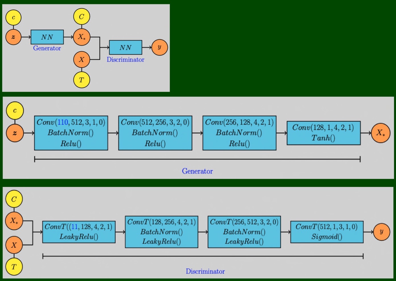
1 今回のモデル
2 準備
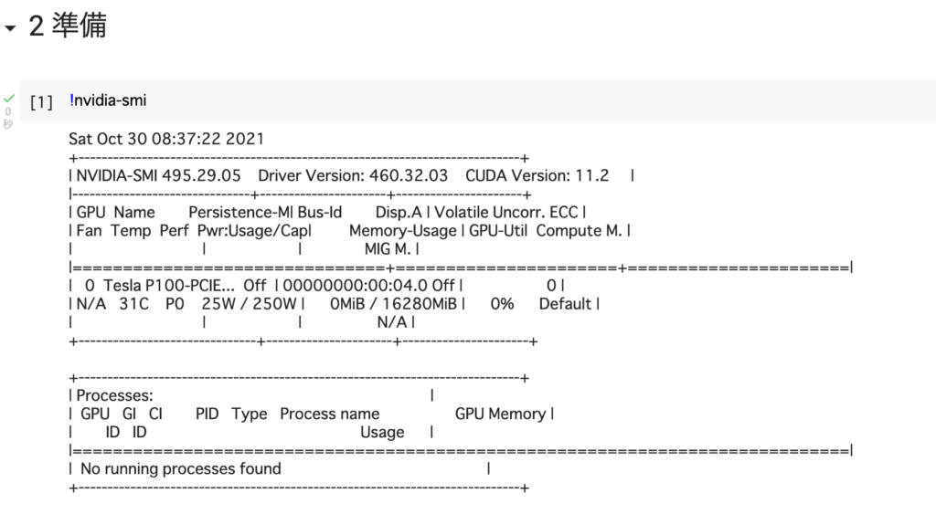
# [1]
!nvidia-smi
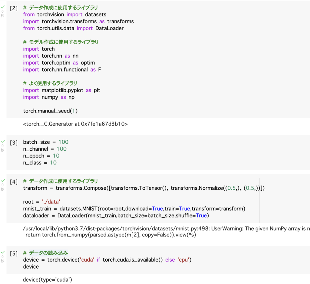
# [2]
# データ作成に使用するライブラリ
from torchvision import datasets
import torchvision.transforms as transforms
from torch.utils.data import DataLoader
# モデル作成に使用するライブラリ
import torch
import torch.nn as nn
import torch.optim as optim
import torch.nn.functional as F
# よく使用するライブラリ
import matplotlib.pyplot as plt
import numpy as np
torch.manual_seed(1)
# [3]
batch_size = 100
n_channel = 100
n_epoch = 10
n_class = 10
# [4]
# データ作成に使用するライブラリ
transform = transforms.Compose([transforms.ToTensor(), transforms.Normalize((0.5,), (0.5,))])
root = './data'
mnist_train = datasets.MNIST(root=root,download=True,train=True,transform=transform)
dataloader = DataLoader(mnist_train,batch_size=batch_size,shuffle=True)
# [5]
# データの読み込み
device = torch.device('cuda' if torch.cuda.is_available() else 'cpu')
device
3 モデル
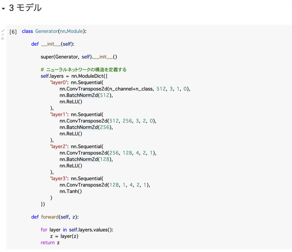
# [6]
class Generator(nn.Module):
def __init__(self):
super(Generator, self).__init__()
# ニューラルネットワークの構造を定義する
self.layers = nn.ModuleDict({
'layer0': nn.Sequential(
nn.ConvTranspose2d(n_channel+n_class, 512, 3, 1, 0),
nn.BatchNorm2d(512),
nn.ReLU()
),
'layer1': nn.Sequential(
nn.ConvTranspose2d(512, 256, 3, 2, 0),
nn.BatchNorm2d(256),
nn.ReLU()
),
'layer2': nn.Sequential(
nn.ConvTranspose2d(256, 128, 4, 2, 1),
nn.BatchNorm2d(128),
nn.ReLU()
),
'layer3': nn.Sequential(
nn.ConvTranspose2d(128, 1, 4, 2, 1),
nn.Tanh()
)
})
def forward(self, z):
for layer in self.layers.values():
z = layer(z)
return z
# [7]
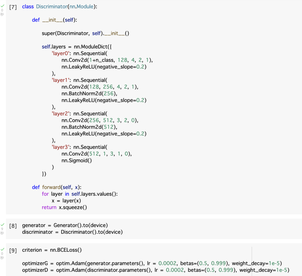
class Discriminator(nn.Module):
def __init__(self):
super(Discriminator, self).__init__()
self.layers = nn.ModuleDict({
'layer0': nn.Sequential(
nn.Conv2d(1+n_class, 128, 4, 2, 1),
nn.LeakyReLU(negative_slope=0.2)
),
'layer1': nn.Sequential(
nn.Conv2d(128, 256, 4, 2, 1),
nn.BatchNorm2d(256),
nn.LeakyReLU(negative_slope=0.2)
),
'layer2': nn.Sequential(
nn.Conv2d(256, 512, 3, 2, 0),
nn.BatchNorm2d(512),
nn.LeakyReLU(negative_slope=0.2)
),
'layer3': nn.Sequential(
nn.Conv2d(512, 1, 3, 1, 0),
nn.Sigmoid()
)
})
def forward(self, x):
for layer in self.layers.values():
x = layer(x)
return x.squeeze()
# [8]
generator = Generator().to(device)
discriminator = Discriminator().to(device)
# [9]
criterion = nn.BCELoss()
optimizerG = optim.Adam(generator.parameters(), lr = 0.0002, betas=(0.5, 0.999), weight_decay=1e-5)
optimizerD = optim.Adam(discriminator.parameters(), lr = 0.0002, betas=(0.5, 0.999), weight_decay=1e-5)
4 条件指定用関数
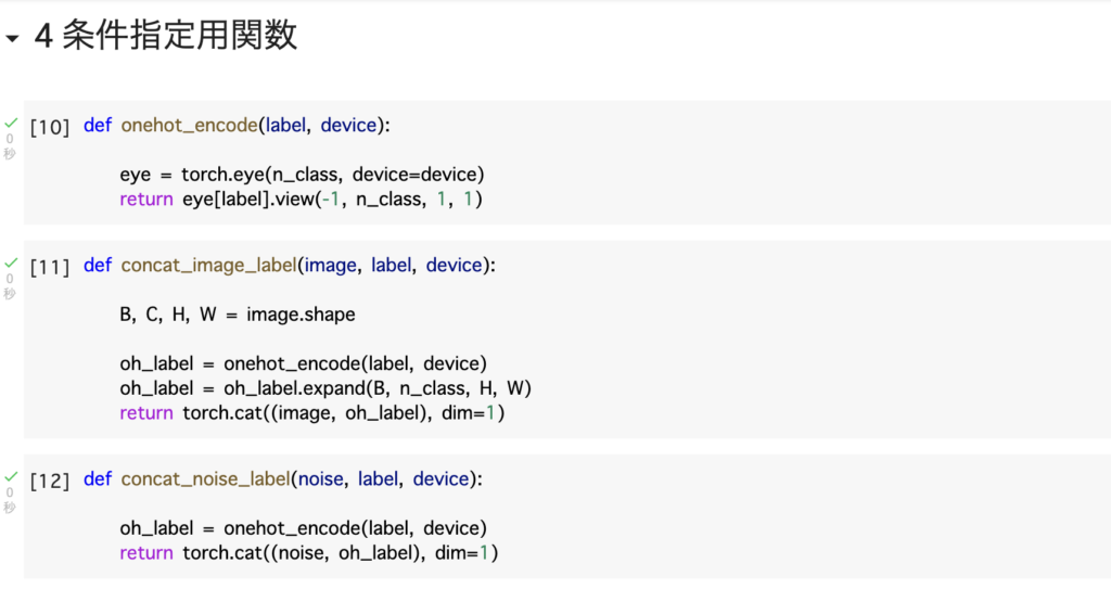
# [10]
def onehot_encode(label, device):

    eye = torch.eye(n_class, device=device)
    return eye[label].view(-1, n_class, 1, 1)

# [11]
def concat_image_label(image, label, device):

    B, C, H, W = image.shape

    oh_label = onehot_encode(label, device)
    oh_label = oh_label.expand(B, n_class, H, W)
    return torch.cat((image, oh_label), dim=1)

# [12]
def concat_noise_label(noise, label, device):

    oh_label = onehot_encode(label, device)
    return torch.cat((noise, oh_label), dim=1)
5 モデルの学習
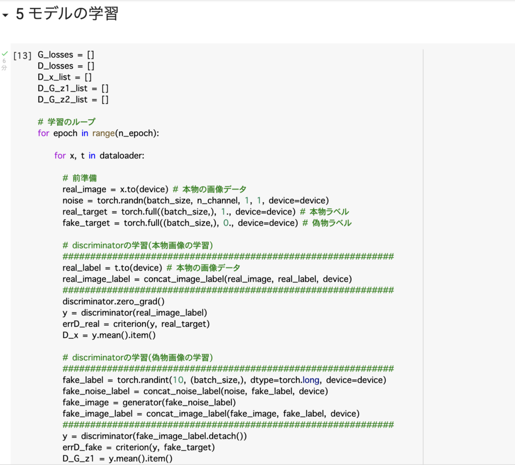
# [13]
G_losses = []
D_losses = []
D_x_list = []
D_G_z1_list = []
D_G_z2_list = []
# 学習のループ
for epoch in range(n_epoch):
for x, t in dataloader:
# 前準備
real_image = x.to(device) # 本物の画像データ
noise = torch.randn(batch_size, n_channel, 1, 1, device=device)
real_target = torch.full((batch_size,), 1., device=device) # 本物ラベル
fake_target = torch.full((batch_size,), 0., device=device) # 偽物ラベル
# discriminatorの学習(本物画像の学習)
############################################################
real_label = t.to(device) # 本物の画像データ
real_image_label = concat_image_label(real_image, real_label, device)
############################################################
discriminator.zero_grad()
y = discriminator(real_image_label)
errD_real = criterion(y, real_target)
D_x = y.mean().item()
# discriminatorの学習(偽物画像の学習)
############################################################
fake_label = torch.randint(10, (batch_size,), dtype=torch.long, device=device)
fake_noise_label = concat_noise_label(noise, fake_label, device)
fake_image = generator(fake_noise_label)
fake_image_label = concat_image_label(fake_image, fake_label, device)
############################################################
y = discriminator(fake_image_label.detach())
errD_fake = criterion(y, fake_target)
D_G_z1 = y.mean().item()
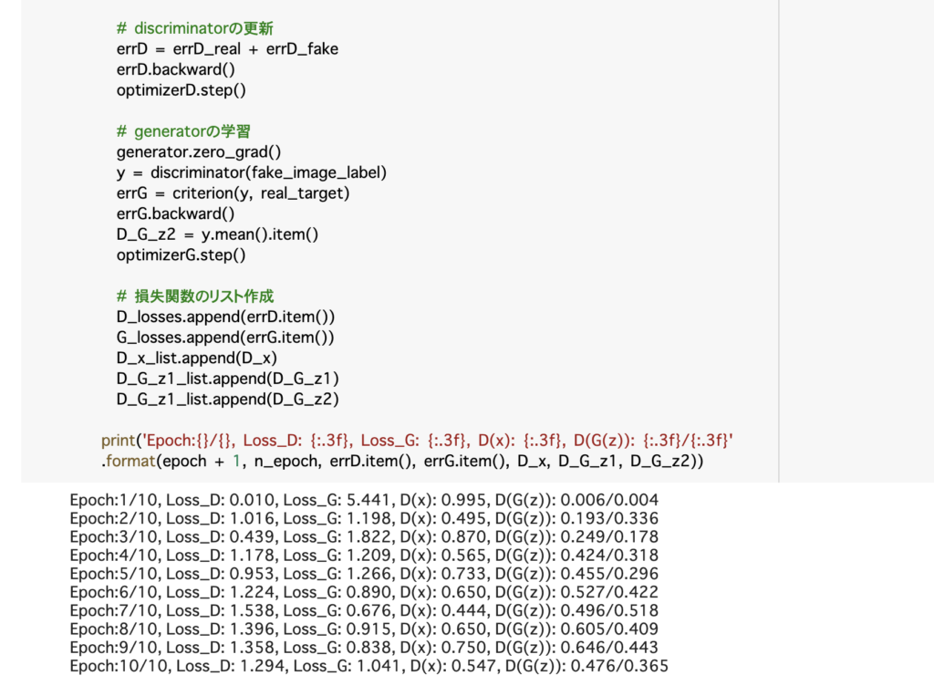
# discriminatorの更新
errD = errD_real + errD_fake
errD.backward()
optimizerD.step()
# generatorの学習
generator.zero_grad()
y = discriminator(fake_image_label)
errG = criterion(y, real_target)
errG.backward()
D_G_z2 = y.mean().item()
optimizerG.step()
# 損失関数のリスト作成
D_losses.append(errD.item())
G_losses.append(errG.item())
D_x_list.append(D_x)
D_G_z1_list.append(D_G_z1)
D_G_z1_list.append(D_G_z2)
print('Epoch:{}/{}, Loss_D: {:.3f}, Loss_G: {:.3f}, D(x): {:.3f}, D(G(z)): {:.3f}/{:.3f}'
.format(epoch + 1, n_epoch, errD.item(), errG.item(), D_x, D_G_z1, D_G_z2))
6 画像の生成
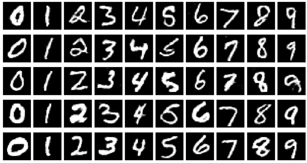
# [14]
# サンプルデータの作成
sample_noise = torch.randn(batch_size, n_channel, 1, 1, device=device)
sample_label = [i for i in range(10)] * (batch_size // 10)
sample_label = torch.tensor(sample_label, dtype=torch.long, device=device)
sample_noise_label = concat_noise_label(sample_noise, sample_label, device)
generator.eval
y = generator(sample_noise_label)

# データの可視化
fig = plt.figure(figsize=(20,20))
plt.subplots_adjust(wspace=0.1, hspace=-0.8)
for i in range(50):
  ax = fig.add_subplot(5, 10, i+1, xticks=[], yticks=[])
  ax.imshow(y[i,].view(28,28).cpu().detach(), "gray")